Algebra

Automatic manipulation of algebraic expressions is a fascinating example of a field in which Maxima draws on a collection of mathematical knowledge implemented over a period of decades. To avoid tripping over what – at first glance – appears to be a quirky approach to sorting variables in the output, you might want to take control of how the variables are output. The following example uses the variables a, b, c, d, x, y, and z. The command ordergre-at(a,b,c,d,x,y,z) forces this order in the output. When you type

Maxima displays the expression in a visually attractive way:

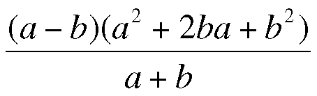
Like other CAS systems, wxMaxima supports methods that apply mathematical laws to simplify algebraic expressions, typically by means of sophisticated rephrasing and reducing. The example here uses the ratsimp(%) command. wxMaxima identifies the binomial formula, converts appropriately, and reduces the results to a very simple expression a2 * b2.

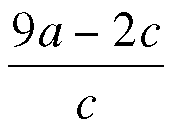
wxMaxima shows ((9*a-c)/c)+((7*a-2*b)/(2*b-7*a)) as:

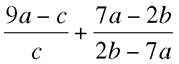
Calling the Ratsimp simplification method creates the following equivalent expression:

Graphical output of function curves (plotting) is another useful feature. wxMaxima relies on the popular Gnuplot package for plotting. To access the Plot menu, you have two options. The top menu bar includes a number of useful subitems below Plot, but you can just as easily press the 2D Plot button in the lower part of the screen. The top line of the dialog expects the function to plot: 4*x2+7. You can leave the other settings as is for the time being. Clicking OK displays the graph shown in Figure 1.

In many cases, a user might want to simply change a couple of graphics parameters. A simple trick to avoid the need to enter the same values time and time again in the dialog is clicking the line that produced the last plot command to tell the plot function to apply the same values the next time you call it. Then you can change the values individually.

Graphical Output

Some functions with two independent variables result in interesting graphs. The 3D Plot menu item lets you plot three-dimensional graphs. The example in Figure 2 shows the output of the function cos(sqrt(5*x2 + 3*y2)). In this case, it makes sense to choose the Openmath output format. This not only opens a new window for the graph but lets you use the mouse to rotate, zoom, and scale the output (Figure 3).

Optimization

Maxima is not just a tool for mathematical experiments; it can help you solve genuine problems, as the next simple example shows.

For an example of Maxima in the real world, consider a chemical manufacturer who produces two liquid products (P1 and P2), which are sold with different profit margins (PM-P1 = EUR 95 and PM-P2 = EUR 75). Both products are made up of four component products (C1 to C4) – these component products might represent color components.

A precisely defined mixing ratio is required for both of the products: the vector P1(3; 1; 3; 11) specifies that to produce one unit (UN) of P1, exactly three units of V1 are required, whereas just one UN of V2 is required. The vector for the other product is P2(1; 5; 2; 2). The example also assumes that resources of the component products are limited. The plan thus needs to take the existing stocks S of the component products into consideration: S(260; 575; 320; 920).

On the basis of this data, it is possible to generate a mathematical model, which Maxima can solve by linear optimization. The first thing is to define the target function. It is safe to assume that the planner will want to maximize the profit margins generated by P1 and P2:

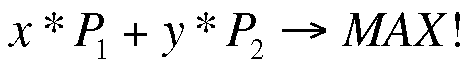
The values x and y represent the number of units to produce. The remaining details in this example are defined as auxiliary conditions that ensure the solution is physically possible. In the case of component product C1, each unit of P1 will consume exactly three units of C1. On the basis of the same system, each unit of P2 consumes one unit of C1, and so on. Because only 260 units of C1 exist, the first auxiliary condition is:

On the basis of the same reasoning, you can apply three further auxiliary conditions. First, add two more to prevent x and y from assuming negative values, because a negative quantity can't exist in real conditions in many situations:

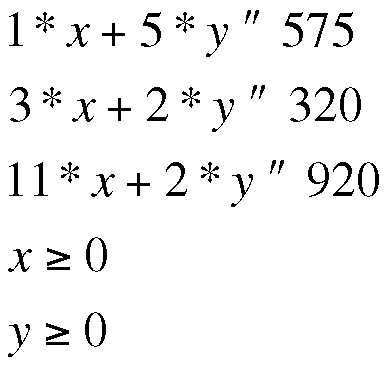
Figure 4 shows the coherencies: the polygon between the x and y axes and the colored straight lines containing all possible combinations of solution for optimizing production. The most favorable combination will be at the top, far right. The black target function is drawn to intersect some of the auxiliary conditions at the optimum point, and you want Maxima to calculate this point.

To simplify changes, all the details are stored as variables:

Tf: 95*x + 75*y
Con1: 3*x + y <= 260
Con2: 1*x + 5*y <= 575
Con3: 3*x + 2*y <= 320
Con4: 11*x + 2*y <= 920
Con5: x >= 0
Con6: y >= 0

As the first step toward an optimized solution, you first need to load the Simplex module using the Maxima load(simplex) command. Then you can call the function maximize_sx(Tf; [Con1;Con2;Con3;Con4;Con5;Con6]) and pass in the target function and the auxiliary conditions to it. The results show that producing 34.6 units of P1 and 108 units of P2 would result in the perfect profit margin of EUR 11,394. The Maxima manual still refers to this function as maximize_lp(); however, maximize_sx() replaced it years ago. In a similar way, the minimize_sx() function handles minimization. The Simplex method implemented by Maxima is extremely powerful.

The number of variables and auxiliary conditions can be very large, again depending on the amount of RAM you have available. This puts relatively small computers with the free Maxima program in a position to solve optimization tasks that would have kept a mainframe busy for hours just 20 years ago.