Choosing the best alternative with topsis-python

Better Decisions

© Photo by Jon Tyson on Unsplash

© Photo by Jon Tyson on Unsplash

Article from Issue 242/2021
Author(s):

Complex decisions require the evaluation of multiple criteria. This article shows how to support such decisions with Linux, Python, and the TOPSIS Multi-Criteria Decision Model.

Zoning is the process by which a city's authorities define the type of land use that will be allowed in different areas of the city. Some of the zoning objectives include the promotion of tourism, employment, safety, and the general well-being of communities. As you might expect, the zoning process generates disputes due to different interests and visions.

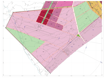
For example, some residents might prefer to locate the industrial zone on the periphery, and others might want it in the center of the city. Which is better? The answer depends on multiple factors (Figure 1). For example, the city of Lyon, France, had its industries located in the periphery. When it suffered a strong economic collapse in the second half of the 20th century, it found itself with a deteriorated and dangerous area that needed a strong investment to be recovered. The opposite was true of Manchester, England, which had an industrial zone in the heart of the city. During the economic crisis of the 1930s, depressed industries degraded and devalued downtown properties.

Figure 1: Atypical zoning proposal (Arica, Chile. Public domain).

Because zoning decisions affect cities for decades, an objective methodology is needed to evaluate both qualitative and quantitative factors. One evaluation option is Multi-Criteria Decision Models (MCDMs).

MCDMs are models that compare multiple decision alternatives, considering both qualitative and quantitative variables. These models provide an ordered list of alternatives, from the best/optimal to the least desirable.

Several MCDM models exist. In fact, planners often use more than one model and then compare the results. One example of an MCDM model that lends itself to easy computer analysis is Technique for Order of Preference by Similarity to Ideal Solution (TOPSIS). A ready-made Python module called topsis-python makes it especially convenient to apply TOPSIS techniques.

TOPSIS is used every day to evaluate multi-million dollar civic improvement projects. However, if you like to code and are interested in the possibility of applying advanced analysis tools to everyday decisions, you can find a way to use TOPSIS for much simpler tasks, such as helping you determine where to buy a house or where to go on vacation. This article introduces you to the TOPSIS analysis process and puts TOPSIS to work on a simple comparison problem.

About TOPSIS

The TOPSIS technique was developed by Hwang and Yoon in 1981 [1]. The goal of TOPSIS is to find the positive ideal solution (which maximizes benefits and minimizes costs) and the negative ideal solution (which minimizes benefits and maximizes costs). TOPSIS also calculates the alternative that simultaneously has the shortest distance from the positive ideal solution and the longest distance from the negative ideal solution.

To better explain the TOPSIS technique, take a look at Figure 2. Suppose you must select a Linux distribution to install on your new computer. There are five possible alternatives (A1, A2, A3, A4, and A5). These alternatives are evaluated with two criteria: Popularity/market share (M) and Number of available packages (P).

Figure 2: The TOPSIS technique.

You can see that the highest possible value for the criterion Popularity/market share (M) is in the alternative A5, and the best value for the criterion Number of available packages (P) is the alternative A1. Then an ideal alternative would be one that combines these two values, which I call the Ideal solution (I in Figure 2). In the same way, I will define the point with the lowest possible values of both criteria and will call it the Anti-ideal solution (AI).

Because in the example (and in most real cases) no alternative fulfills all the requirements of the ideal solution, TOPSIS tells us that the best alternative is the one that simultaneously has the shortest euclidean distance to the ideal solution and the longest to the anti-ideal solution. To reach this solution, TOPSIS makes calculations in 6 steps (see the box entitled "TOPSIS Steps") [2].

TOPSIS Steps

Step 1: Calculate the normalized decision matrix

The first step is to bring the values of the criteria of each alternative to common units. Although TOPSIS does not require the use of a specific normalization procedure, vector normalization is generally used.

Step 2: Calculate the weighted normalized decision matrix

In the second step, each normalized value is weighted by the importance given. This definition of weights or importance is subjective. (In real cases, these weights are defined by a commission of external experts.)

Step 3: Determine the ideal and anti-ideal solutions

The third step is the calculation of the ideal (A*) and anti-ideal (A-) solution. For cases where the criterion is a benefit, the ideal solution is the maximum value of the normalized matrix, and the minimum value will be the anti-ideal. In cases where the criterion is a cost (or value to be minimized), the ideal solution will be the minimum value and the anti-ideal the maximum value.

Step 4: Calculate the separation measures

The fourth step is to calculate the distance of each alternative to the ideal solution (Di*) and the distance of each alternative to the anti-ideal solution (Di-).

Step 5: Calculate the relative closeness to the ideal solution

The relative closeness (Ci*) takes values between 0 and 1. Alternatives closer to 1 are closer to the ideal solution, and alternatives closer to 0 are closer to the anti-ideal.

Step 6: Rank the alternatives

Finally, from the relative proximity, the alternatives are ranked; the most recommended is the one that is closest to the ideal solution and farthest from the anti-ideal solution.

An Example

Assume you wish to define the city's optimal zone to install industries. The possible alternatives are shown in Table 1. Table 1 also shows the criteria that will be used to evaluate the alternatives (including an indication of whether the criteria seeks to maximize or minimize). The criteria are:

  • C1: Cost to relocate a company that is out of the area; minimization is sought (Min).
  • C2: Expected level of employment if the zone is selected; maximization is sought (Max).
  • C3: Negative externalities generated (e.g., noise); minimization is sought (Min).
  • C4: Positive impact on the social development of the area; maximization is sought (Max).

Table 1

Alternatives and Evaluation Criteria

Alternatives

C1

C2

C3

C4

A1

3.0

100

10

7

A2

2.5

80

8

5

A3

1.8

50

20

1

A4

2.2

70

12

9

Seeking

Min

Max

Min

Max

The criteria are not all equally important, so I will give them different weights. In real cases, a commission of independent experts will assign the weights, but for this example, I will define the weights of the criteria as follows (on a scale from 0 to 1, where 0 means "unimportant" and 1 means "the most important"):

C1: 0.188
C2: 0.266
C3: 0.135
C4: 0.411

To find the solution to the problem, I will use Python 3 on Ubuntu with the topsis-python module.

The first step is to open the command line and install the module [3] (Figure 3):

pip3 install topsis-jamesfallon
Figure 3: Installing topsis-python.

After installing the module, use the Python interpreter to enter the problem data (Listing 1). Variable "a" represents the alternatives/criteria values (also knows as decision matrix). Variable "w" stores the assigned weights of the criteria. The information on minimization/maximization is provided in "I" (Figure 4).

Listing 1

Inputting the Data

>>> from topsis import topsis
>>> a = [[3, 100, 10, 7], [2.5, 80, 8, 5], [1.8, 50, 20, 11], [2.2, 70, 12, 9]]
>>> w = [0.188, 0.266, 0.135, 0.411]
>>> I = [0, 1, 0, 1]
>>> decision = topsis(a, w, I)
Figure 4: Use the Python interpreter to execute the steps from the command line.

Once you have input the data, the functions of the topsis-python module will perform the necessary calculations. If you want to skip directly to the final answer, calling decision.calc() executes all the steps at once, and decision.optimum_choice returns the optimal alternative (Figure 5). However, if you're interested in the intermediate calculations, topsis-python has separate functions that execute each of the TOPSIS steps (refer to the box entitled "TOPSIS Steps"). As shown in Listing 2, you can start by using the decision.step1 function and the decision.r variable to calculate the normalized decision matrix (Table 2).

Figure 5: Finding the optimum choice.

Listing 2

Normalized Decision Matrix

>>> decision.step1
>>> decision.r
array([[0.62110337, 0.51758614, 0.37266202, 0.4554758 ],
       [0.64820372, 0.51856298, 0.32410186, 0.45374261],
       [0.37582301, 0.30065841, 0.75164603, 0.45098762],
       [0.42135049, 0.30096463, 0.66212219, 0.54173634]])

Table 2

Normalized Decision Matrix

Alternatives

C1

C2

C3

C4

A1

0.62110337

0.51758614

0.37266202

0.4554758

A2

0.64820372

0.51856298

0.32410186

0.45374261

A3

0.37582301

0.30065841

0.75164603

0.45098762

A4

0.42135049

0.30096463

0.66212219

0.54173634

Then decision.step2 multiplies the normalized decision matrix by the weight associated with each of the criteria to determine the weighted normalized decision matrix (Listing 3, Table 3). As shown in Listing 4, the decision.step3 function puts the ideal solution in the decision.ab variable and the anti-ideal solution in decision.aw (Table 4). In Listing 5, decision.step4 calculates the separation measure to the ideal solution (decision.db) and the negative-ideal solution (decision.dw) – the results appear in Table 5. Use decision.step5 and decision.C to calculate the relative closeness to the ideal solution (Listing 6, Table 6), then finally call the decision.C variable to get the ranking of the alternatives (Listing 7, Table 7).

Listing 3

Weighted Normalized Decision Matrix

>>> decision.step2
>>> decision.v
array([[0.11676743, 0.09730619, 0.07006046, 0.08562945],
       [0.17242219, 0.13793775, 0.0862111 , 0.12069553],
       [0.05073611, 0.04058889, 0.10147221, 0.06088333],
       [0.17317505, 0.12369646, 0.27213222, 0.22265364]])
>>>

Table 3

Weighted Normalized Decision Matrix

Alternatives

C1

C2

C3

C4

A1

0.11676743

0.09730619

0.07006046

0.08562945

A2

0.17242219

0.13793775

0.0862111

0.12069553

A3

0.05073611

0.04058889

0.10147221

0.06088333

A4

0.17317505

0.12369646

0.27213222

0.22265364

Listing 4

Ideal and Anti-Ideal Solutions

>>> decision.step3
>>> decision.ab
array([0.07006046, 0.17242219, 0.04058889, 0.27213222])
>>> decision.aw
array([0.11676743, 0.0862111 , 0.10147221, 0.12369646])
>>>

Table 4

Ideal and Anti-Ideal Solutions


C1

C2

C3

C4

Positive ideal solution

0.07006046

0.17242219

0.04058889

0.27213222

Negative ideal solution

0.11676743

0.0862111

0.10147221

0.12369646

Listing 5

Separation Measures

>>> decision.step4
>>> decision.db
array([0.10989554, 0.1548053 , 0.10554209, 0.07601339])
>>> decision.dw
06 array([0.11160034, 0.08222631, 0.15561078, 0.11661359])
>>>

Table 5

Separation Measures

 >

A1

A2

A3

A4

Distance to the ideal solution

0.10989554

0.1548053

0.10554209

0.07601339

Distance to the anti-ideal solution

0.11160034

0.08222631

0.15561078

0.11661359

Listing 6

Relative Closeness to the Ideal Solution

>>> decision.step5
>>> decision.C
array([0.50384838, 0.3469002 , 0.59586089, 0.60538555])
>>> decision.optimum_choice
3
>>>

Table 6

Relative Closeness to the Ideal Solution


A1

A2

A3

A4

Relative Closeness

0.50384838

0.3469002

0.59586089

0.60538555

Listing 7

Ranking the Alternatives

>>> decision
Best alternative
a[3]: [ 2.2 70.  12.   9. ]
>>> decision.C
array([0.50384838, 0.3469002 , 0.59586089, 0.60538555])

Table 7

Ranking the Alternatives

Alternative

Result

Rank

A4

0.60538555

1

A3

0.59586089

2

A1

0.50384838

3

A2

0.3469002

4

According to the result in Listing 7, the optimal alternative, that is, the one that maximizes the benefits and minimizes the negative externalities, is number 4 (array position 3). In addition, the result shows that the second best alternative is number 3, then number 1, and finally number 2.

Conclusion

In real-world scenarios, the number of criteria and alternatives is higher, but this example shows how to define complex problems and obtain an optimal decision in a simple way using Python, Linux, and TOPSIS.

Infos

  1. Hwang, C.L. and K. Yoon. Multiple Attribute Decision Making: Methods and Applications. Springer-Verlag, New York, 1981
  2. Papathanasiou, J. and N. Ploskas. "TOPSIS". In: Multiple Criteria Decision Aid. Springer Optimization and Its Applications, vol. 136. Springer, Cham, 2018: https://doi.org/10.1007/978-3-319-91648-4_1
  3. topsis-python module: https://pypi.org/project/topsis-jamesfallon/

The Author

Juan Tobar has worked as an advisor to local governments and the Chilean Congress, as well as a university professor and FLOSS software developer. He is currently researching the relationship between public investment and citizen satisfaction through the use of Cellular Automata and MCDMs for CorporaciÛn de Desarrollo de Tarapac· and Consultores TyT in Chile. For more information: mailto:juan.tobar@consultorestyt.com.

Buy this article as PDF

Express-Checkout as PDF
Price $2.95
(incl. VAT)

Buy Linux Magazine

SINGLE ISSUES
 
SUBSCRIPTIONS
 
TABLET & SMARTPHONE APPS
Get it on Google Play

US / Canada

Get it on Google Play

UK / Australia

Related content

comments powered by Disqus
Subscribe to our Linux Newsletters
Find Linux and Open Source Jobs
Subscribe to our ADMIN Newsletters

Support Our Work

Linux Magazine content is made possible with support from readers like you. Please consider contributing when you’ve found an article to be beneficial.

Learn More

News