Request Spotify dossiers and evaluate them with Go and R
Streaming services such as Spotify or Apple Music dominate the music industry. Their extensive catalogs now cover the entire spectrum of consumable music. Relying on artificial intelligence, these services introduce users to new songs they'll probably like, as predicted by the services' algorithms. Traditional physical music media no longer stand a chance against this and gather dust on the shelves. Of course, this development also means that anonymous music consumption is a thing of the past, because streaming services keep precise records of who played what track, when, and for how long.
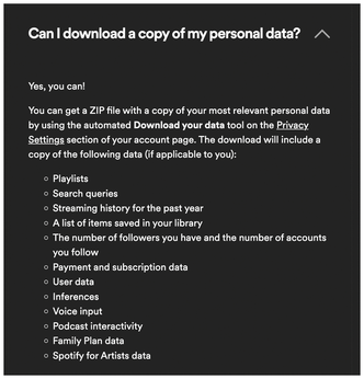
On request, Spotify will even hand over the acquired data (Figure 1). If you poke around a bit on their website, you'll find the buttons you need to press to request a copy of these files in Account | Privacy Settings, but Spotify takes their sweet time to respond. From the time of the request, it takes about a week for their archivist to retrieve the data from the files in the Spotify basement, compress them, and post them as a ZIP archive on the website for you to pick up. After receiving Spotify's email notification, you can then download the data for two weeks and poke around in it locally to your heart's content.
[...]
Buy this article as PDF
(incl. VAT)