Backdoors in Machine Learning Models
Interest in machine learning has grown incredibly quickly over the past 20 years due to major advances in speech recognition and automatic text translation. Recent developments (such as generating text and images, as well as solving mathematical problems) have shown the potential of learning systems. Because of these advances, machine learning is also increasingly used in safety-critical applications. In autonomous driving, for example, or in access systems that evaluate biometric characteristics. Machine learning is never error-free, however, and wrong decisions can sometimes lead to life-threatening situations. The limitations of machine learning are very well known and are usually taken into account when developing and integrating machine learning models. For a long time, however, less attention has been paid to what happens when someone tries to manipulate the model intentionally.
Adversarial Examples
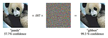
Experts have raised the alarm about the possibility of adversarial examples [1] – specifically manipulated images that can fool even state-of-the-art image recognition systems (Figure 1). In the most dangerous case, people cannot even perceive a difference between the adversarial example and the original image from which it was computed. The model correctly identifies the original, but it fails to correctly classify the adversial example. Even the category in which you want the adversial example to be erroneously classified can be predetermined. Developments [2] in adversarial examples have shown that you can also manipulate the texture of objects in our reality such that a model misclassifies the manipulated objects – even when viewed from different directions and distances.
[...]
Buy this article as PDF
(incl. VAT)
Buy Linux Magazine
US / Canada
UK / Australia
Subscribe to our Linux Newsletters
Find Linux and Open Source Jobs
Subscribe to our ADMIN Newsletters
Support Our Work
Linux Magazine content is made possible with support from readers like you. Please consider contributing when you’ve found an article to be beneficial.

News
-
Plasma Ends LTS Releases
The KDE Plasma development team is doing away with the LTS releases for a good reason.
-
Arch Linux Available for Windows Subsystem for Linux
If you've ever wanted to use a rolling release distribution with WSL, now's your chance.
-
System76 Releases COSMIC Alpha 7
With scores of bug fixes and a really cool workspaces feature, COSMIC is looking to soon migrate from alpha to beta.
-
OpenMandriva Lx 6.0 Available for Installation
The latest release of OpenMandriva has arrived with a new kernel, an updated Plasma desktop, and a server edition.
-
TrueNAS 25.04 Arrives with Thousands of Changes
One of the most popular Linux-based NAS solutions has rolled out the latest edition, based on Ubuntu 25.04.
-
Fedora 42 Available with Two New Spins
The latest release from the Fedora Project includes the usual updates, a new kernel, an official KDE Plasma spin, and a new System76 spin.
-
So Long, ArcoLinux
The ArcoLinux distribution is the latest Linux distribution to shut down.
-
What Open Source Pros Look for in a Job Role
Learn what professionals in technical and non-technical roles say is most important when seeking a new position.
-
Asahi Linux Runs into Issues with M4 Support
Due to Apple Silicon changes, the Asahi Linux project is at odds with adding support for the M4 chips.
-
Plasma 6.3.4 Now Available
Although not a major release, Plasma 6.3.4 does fix some bugs and offer a subtle change for the Plasma sidebar.